The Plantation Thinning Simulator Method
Introduction: Why Thin?
Why bother to thin a Black Walnut plantation at all? A good question. Regarding tree density, it has been noted that trees generate the same volume of wood per year per acre no matter how many trees there are. The annual volume addition to total salable timber boles might be 150 to 500 board feet per year per acre of canopy, depending on the site. So, is it better to add a little of that annual volume to a lot of small crown slow growing trees or divide that annual volume among to a few big crown, and hence, faster growing trees? Does it make any economic difference where the volume is added?
The answer has to do with pricing, health, and life span, both for trees and land owners. For a Black Walnut trees, health seems to peak at about 110 years. The trees may stay alive and grow for another 100 years, but they start falling apart on the inside. The peak timber value, of course, is during the hump, and big logs, not only have big volumes, they fetch a lot more per board foot than small logs. If there was no hard time limit, one could just wait 300 years and the lots of small logs would become lots of big logs and fetch the big price, but the jammed in skinny tree option just runs out of time. Heavily crowded trees cannot live long enough and grow big enough to earn the top veneer price. An unmanaged walnut plantation is a bad idea. For best return, the canopy needs to be maintained intact with the fewest and best trees available, and add the annual volume allowance onto the most expensive logs possible.
Perfect!
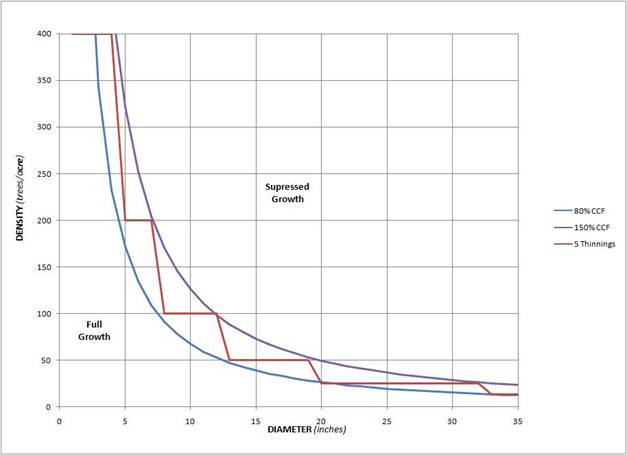
Tree Density Required for Unrestricted Growth and a Plan where Half the Trees are Removed in each of 5 Thinnings
The above diagram shows two important lines, a Crown Competition Factor (CCF) of 80% and 150%. Crown Competition Factor is a measure of tree canopy crowding. (For an explanation of CCF, see Appendix A.) It has been found that with a spacing of 80% CCF trees grow unrestricted for sunlight. A more crowded forest at 150% CCF will restrict each of the twice-too-many trees to about half the volumetric growth rate.
The thinning plan shown in the diagram shows five thinnings. When the CCF reaches 150%, half the trees are removed, which drops the crowding to about 80% CCF. The average diameter usually goes up about an inch during a major thinning, because bigger trees tend to survive the cut. Also it takes a few years for saved trees to reach out into new canopy openings and claim the increased growth rate.
The above thinning plan is just one of many possible approaches. Typically forests are only thinned twice during their life cycle. At the other extreme, an intensive managed plantation might remove some trees every year and maintain the tree density on the 80% CCF path.
In a black walnut plantation the goal is invariably to produce veneer logs. To achieve veneer quality in an even-aged setting requires early pruning for clear boles. Also, avoidance of overcrowding followed by heavy thinning, which results in an unwelcome jump in annual ring spacing, and epicormic sprouting.
More Introduction: Why use the Plantation Thinning Simulator Method?
At state and national Walnut Council meetings we always visit tree plantations. I can only remember one of that multitude of woodland plots that did not need thinning. More than one forester has told us that landowners can’t do thinning. Owners just can’t put the axe to their babies that they have so tenderly nursed and shaped up from little twiglings. Unlike a large natural forest, our orderly plantations consist of only high value trees and are usually intensely managed. We don’t mind spending time there, and if necessary performing improvements every year.
No surprise, our own plantation dearly needs thinning. I started out with a spool of bright orange plastic ribbon on row 17 - looking up. I needed to select (save) about 1 tree out of 5, and any selected crop tree should have an open crown on at least 3 sides. I needed to keep track of 2 or 3 rows at once. Before I got half way across the field, I was out of tape, became completely confused, and gave up. This was a job for a computer! After many revisions (rev 15.1.3 just now) and simplifications, the Thinning Simulator and an associated process have been developed. This method may be a waste of time for an experienced forester, but for a befuddled amateur landowner, it is just the ticket. Just enter data, there are no decisions. It will still be painful to cull a nice straight tree, but the Thinning Simulator process can reduce stress, and lend confidence to this wise, yet challenging activity.
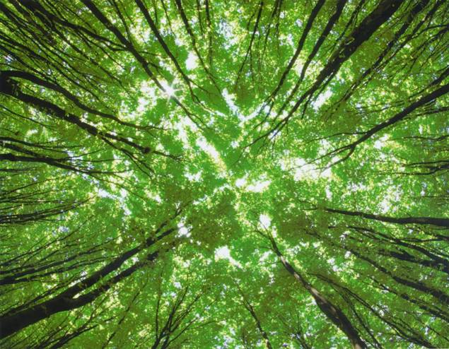
Looking up
The Thinning Simulator Method has the additional bonus of producing accurate thinning results. The software lets a forest manager make program runs that simultaneously includes quantity and quality of each tree and thins the plot to some desired Crown Competition Factor (CCF). If the output looks like too many trees or too few were saved, it is easy to change the target CCF (not so easy to move flags in the planting) and rerun the program to what looks good on the computer screen and then take that printout to the woods. Forest managers can use the software to identify cull trees for early thinnings. Once trees reach marketable size, program can be used to organize a timber sale that keeps the correct number of the best trees for the landowner – Usually with a much different outcome than just turning a logger loose in your woods. The Thinning Simulator process is a decision tool that makes the decisions for us that are so hard to make in the field.
The complete Thinning Simulator Process includes several steps, each of which will be explained in detail. The Thinning Simulator computer program needs the data gathered from the plantation tree plot. Like any computer program it wants the data arranged in a certain fussy way. We will explain and give examples of how to gather, process, and save the data to satisfy the Thinning program’s input requirements.
Once the tree plot data has been read by the simulator program, the user can run thinning scenarios to see the impact of various thinning intensities. After each program run, the number and percent of cull trees is shown along with an expected new growth rate. Competing objectives and issues regarding thinning intensity will be discussed in these instructions. When the user finally gets the intensity wanted for the current thinning, a report can be generated which contains a list of cull trees and the suggested fate of every tree.
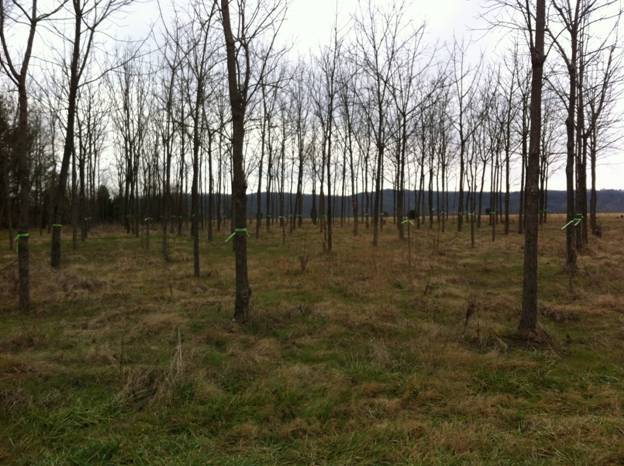
Black Walnut Trees Flagged for Removal
The final two sections of this document discuss how to actually cull trees and what growth rates might expected based on various long term thinning plans. For those interested, optional subjects, and details are relegated to appendixes.
The Walnut Council offers two choices to help its members with their thinning decisions.
1. As a free benefit to its members, the Walnut Council provides a thinning service. Members may request a data collection package, which includes Chapter 1 and 2 of the instructions and blank template data collection forms. Once a member has raw field data in hand, the data is submitted. Volunteers at the Walnut Council will transcribe the data, run the simulator program and reply with the recommended list of trees to cull.
2. As a free benefit to its Life Members, the Walnut Council provides the complete Thinning Simulator software package. Life members may request the complete software package, which comes on a flash drive and includes full instructions, template data forms and spreadsheets, and the Thinning Simulator executable program. Once installed the land owner or researcher can run thinning scenarios on their own computer.
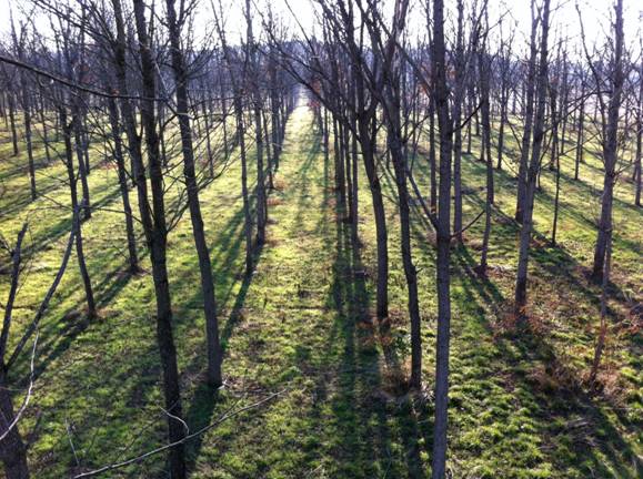
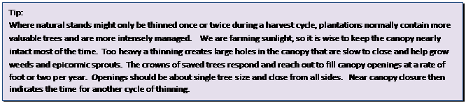
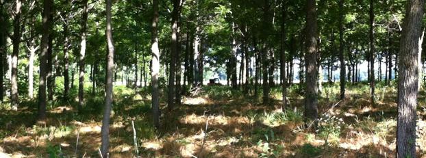
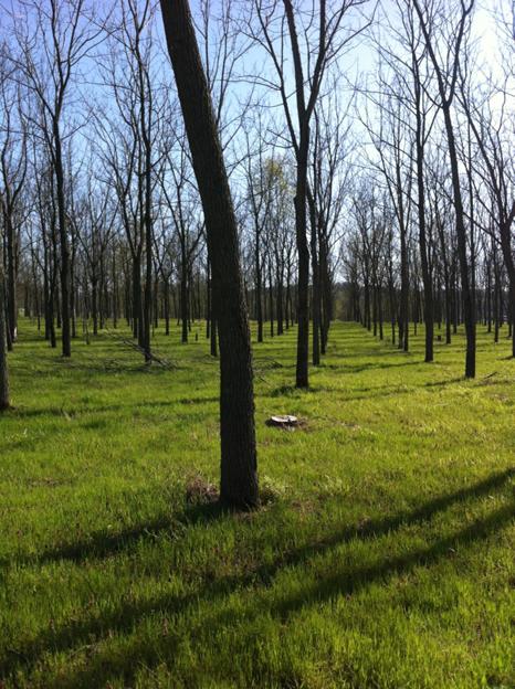
An over-crowded Black Walnut plot
Introduction Why Thin?
Introduction Why use the Plantation Thinning Simulator Method?
Overview Thinning Simulator Method
PART 1 - Collecting Data for the Plantation Thinning Simulator Method
Chapter 1. A Permanent Coordinate System
Chapter 2. Collecting Field Data
PART 2 - Using the Plantation Thinning Simulator Method
Chapter 3. The Distribution Flash Drive Contents
Chapter 4. Entering Field Data into a Sample Spreadsheet
Chapter 5. Computing the Relative Value of each Tree by Formula
Chapter 6. Sort the List of Trees with the Most Valuable Tree on Top.
Chapter 7. Required Header Information and Saving the .csv File
Chapter 8. Using the Thinning Simulator Software.
Chapter 9. Marking Cull Trees
Chapter 10. Removing Cull Trees
Appendix A Crown Competition Factor Explained
Appendix B Tips on Making a Permanent Coordinate System
Appendix C Tips on Collecting Field Data
Appendix D Formula for Computing Tree Value
Appendix E Simulating Average Tree Growth
Appendix Y Possible Uses for Undersized Logs and Waste Material.
Appendix Z The Thinning Simulator Algorithms and Mathematics
Overview: The Plantation Thinning Simulator Method
Walnut Council members may obtain a Thinning Data Collection package from the Walnut Council. The Thinning Data package can be eMailed or downloaded from the Walnut Council website. The package contains a template blank field data collection sheet, sample field data spreadsheet, and instructions. After a coordinate system is established for a plantation plot, the diameter and the length of potential logs are measured and recorded for each tree in the plot. The field measurement data can then be sent to the Walnut Council for analyses, and a report of possible culling actions will be returned.
Life members of the Walnut Council may request the full Thinning Simulator package. The full Thinning Simulator package includes a template blank field data collection sheet, the executable Thinning Simulator program, instructions, and sample plot data files. The field measurement data is entered into a working spreadsheet. A relative value is computed for each tree based on the entered field data. The tree list is then sorted with the best tree on the top of the list, and the list is saved from the working spreadsheet to a file in the required input format to be read by the Thinning Simulator program. The simulator program is started and the input file is selected and loaded into the simulator. Common tree density values are displayed as the plot currently stands. A target Crown Competition Factor (CCF) is changeable and is defaulted to 100%. Usually, several CCF cases are run to see the effect on culling and the percent of trees removed and remaining. Once the user is satisfied with the intensity of the thinning, a report can be saved and printed to be used for tree marking in the field.
PART 1 - Collecting Data for the Thinning Simulator Method
Chapter 1. A Permanent Coordinate System rev 02 2018 Feb 07
Before data can be collected, trees need to be identified. A well-marked Permanent Coordinate System is a nice way to keep track of your trees, but it is downright essential to the Thinning Simulator process. The coordinates not only identify each tree, they tell the simulator where a tree is located and who its neighbors are. Before we begin, some terms that will be used throughout these instructions need to be defined.
For the purposes here, a Plantation is a property where trees are planted (not natural). An owner might own more than one plantation. A Plot is a grid area within a plantation with uniform row and column spacing and a contiguous coordinate system. The simulator deals with one plot at a time. Each tree lives at a permanent coordinate within the plot, and that coordinate is the tree’s permanent name, unless you dig it up and move it. When referring to a tree (like 103-27) the first number is always the Row and the second number is always the tree’s Column. (remember RC Cola?) Rows and columns are identified by whole numbers, not letters. In the field rows and/or columns need not be exactly straight. If trees are planted in rows with random spacing, a land measuring wheel can be used and the column coordinale entered in feet. When drawing a grid, columns always go up and down, just like the Parthenon. The row with the smallest row number is always across the top of the drawing or screen display. There are various ways to permanently mark out rows and columns. We have found that there should be a visible (above the weeds) marker every 10 trees in both directions, or you will spend a lot of time walking. For tips on how to make a permanent coordinate system see Appendix B.
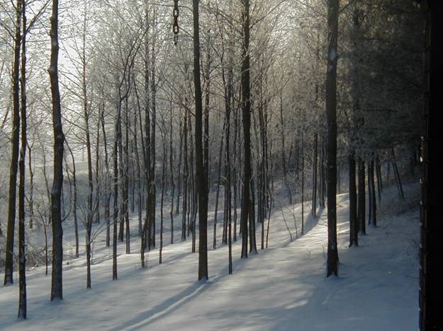
Trees without names. Which trees to cull?
Chapter 2. Collecting Field Data rev 01 2017 Jun 23
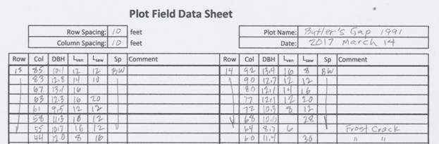
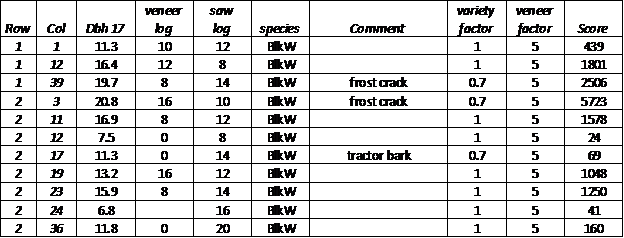
Top part of a typical field data sheet
In collecting field data, the most important item is a tree’s coordinates (Row and Column). The rest of the data items can be a little sloppy, but the tree’s coordinates should be correct.
The next most important data item is the tree’s Diameter Breast High (DBH). The diameter can be guessed, measured with a Biltmore stick, a caliper, or a pi tape. Each respective method is more accurate and slower. The accuracy of guessing DBH is about +- 1.5 inch. A Biltmore stick’s accuracy is about +- 0.5 inch. A caliper’s accuracy is about +- 0.25 inch. A pi tape is good to about +- 0.1 inch. What to use? Consider two good trees side by side and the one with the smaller DBH data recorded (not actual) must go. If you don’t care about a one inch mistake, then guessing DBH is good enough. If you are interested in measuring tree growth, then use a pi tape.
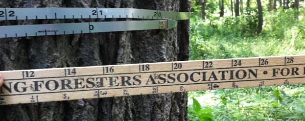
Pi tape above and Biltmore scale below - measuring a 21.1 inch DBH Black Walnut tree
Only a tree’s coordinates, DBH, and the list order are used by the Thinning Simulator program. The data measurements that follow are only used in the spreadsheet to determine a tree’s value for sorting.
To determine a tree’s value we need some measure of its vertical quality. Some users have used Low-Medium-High quality. Others have used numbers 1 to 5. Dr. Walter Beineke has used percent apical. The most rigorous method is to estimate the length of potential veneer and saw logs. Again, for the purpose of the Thinning Simulator, the data is only used to resolve disputes between adjacent trees. Close calls between adjacent trees are not uncommon and more accuracy can settle the argument. The whole Thinning Simulator method needs to be robust enough so there is little second guessing at cull time. The relief of owner’s mental stress is the basic objective of the entire method.
If the plot has mixed species, then a species code should be entered on the data sheet. Other items are entered as comments which might affect the relative value of a tree. For example, frost crack, lean, bird pecks, bark damage, or a special tree.
A template blank Field Data Collection Form is included in the Thinning Simulator distribution packages. The form has entries for veneer and saw log lengths. For tips on collecting data see Appendix C.

Once you have raw field data in hand, you have two choices. You may go through the spreadsheet and Thinning Simulator process described in the following chapters, or you may submit you raw field data to the Walnut Council Thinning Service. As a free benefit to its members, the Walnut Council provides a thinning service. Volunteers will transcribe your data, run the simulator program and reply to you with list of possible culling actions.
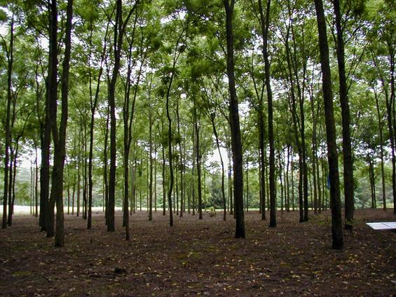
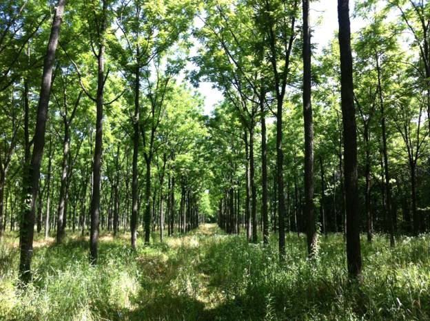
An Intensively Managed Plantation
PART 2 - Using the Thinning Simulator Method
Chapter 3. The Distribution Flash Drive Contents_________________________ rev 01 2018 Jan 01
If you are reading these instructions, you are well on your way in completing the Thinning Simulator Method. The Thinning Method distribution flash drive root directory contains three files: these instructions (Thinning Simulator Method Instructions.doc), a sample field data collection sheet (Field Data Sheet.xls), and the executable Thinning Simulator program (Thinning Simulator.exe).
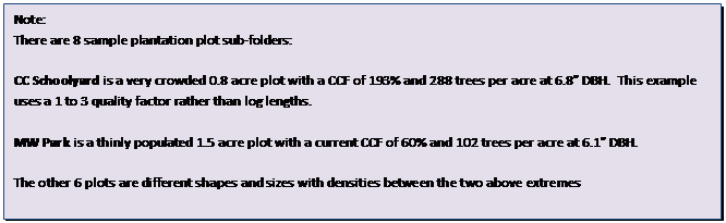
There are several sample plot subdirectories. Each sample plot subdirectory contains a working spreadsheet with a name like (Plantation_Plot_Year.xls). These working spreadsheets are where field data is entered, individual tree values are computed, and the tree list is sorted with the best tree on top. Each sample plot subdirectory also contains a smaller file with a name like (Plantation_Plot_Year.csv). The smaller .csv file is saved from the working spreadsheet in the fussy input format wanted by the Thinning Simulator program.
When running the Thinning Simulator program, you will be asked to select an input .csv files to load. If you want to save a program’s run results, the results are automatically saved in the same directory (folder) from where the input data was loaded.
Chapter 4. Entering Field Data into a Sample Spreadsheet rev 02 2018 Jan 01
Example spreadsheets are included within each sample plot folder on the distribution flash drive. The sample spreadsheets have the file name extension “.xls”, and are readable by Excel and others. Each of the spreadsheet columns will be described as they appear in the sample provided. We like to create a separate file folder for each plantation plot. Copy one of the provided working spreadsheet to your new plot folder and rename the working spreadsheet with an appropriate name. You can erase or overwriting the provided data with your field data.
The following description is going to sound a little like “Who’s on first”, since tree plots have rows and columns and spreadsheets have rows and columns. To maintain sanity the spreadsheet rows will be called “records” and the spreadsheet columns will be called “items”. The data for each tree goes into its own single spreadsheet record. The tree’s plot row number is the 1st item in a record. The tree’s plot column number is the 2nd item in a record , and the tree’s Diameter Breast High (DBH in inches) is the 3rd item in a record. The Thinning Simulator Program only uses these first three data items. The spreadsheet columns after column C are for entering information used to compute a relative value for each tree.
The 4th item is for an estimated veneer log length and item 5 is for a potential saw log length. Item 6 is for species or a variety code and item 7 is for comments. All these data and estimates are from the field data sheets and should have been made in the field as described in Chapter 2, so the data are just entered here without question.
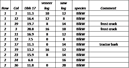
Field Data Entered into a Spreadsheet
Chapter 5. Computing the Relative Value of each Tree by Formula rev 01 2017 Jun 27
The overall goal here is to rank tree in descending owner value with enough accuracy to easily settle arguments between adjacent trees. Feel free to establish tree value any way you like, but you might want to try our way first.
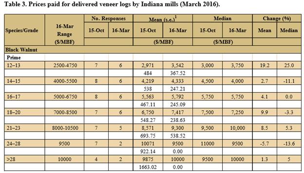
From the field data entered, now we need to compute a relative value for each tree. The Thinning Simulator program expects to read in and favor the best trees first, so the list order is very important. The relative value is only used to sort the tree list, so it need not be anything like actual commercial value. We just need to end up with the best trees on the top of the list. “Value” is a fuzzy and changing concept, so to make things simple we will start out by roughly computing a value proportional to current commercial value. A good source of current commercial log prices is the Indiana Forest Products Price Report. Sawlog and veneer prices are way at the bottom.
Factors and Value Score Added
In spreadsheet record item 8 enter a “variety factor”, which is a multiplier to compare species sawlog prices. If the mean of No.1 black walnut sawlog price is defined as 1.0, then: pine and beech are about .3; red oak, soft maple, tulip poplar, and hickory are about .4; red oak, and ash are about .5; and about .6 for cherry, white oak, and hard maple. Enter the variety factor in item 8 by looking at the species code in item 6. There are two caveats to this entry. If you have a pet tree, or variety, enter a high variety factor to move them up the sorted list and thus be given plot priority. A second adjustment should be made for tree health. From the field comments entered in item 7, enter deductions for health issues. For example, a large tractor damage may not affect the value of a tree now, but you might not want to save such a tree as a final crop tree, since it will probably be a hollow tree at maturity. We give a .7 variety factor to frost cracked and large tractor damaged trees. If you want rid of such trees, give them a .1 and they will be culled for sure.
Spreadsheet record item 9 is a “veneer factor” which is a multiplier to compare veneer price to sawlog price. The factor has been about 5 for walnut and cherry and about 3 for red and white oak. For species without a veneer market, use 1.0, because everything will be sawlogs.
In
spreadsheet record item 10 is the formula to compute the relative tree
value. The issues in developing the value formula can be complex. If you want
to delve into these issues go to Appendix D, otherwise just use the formula
provided in item 10 of the sample working spreadsheets. The formula provided
is proportional to volume for large , gradually favors height for pole sized
trees.
Chapter 6. Sort the List of Trees with the Most Valuable Tree on Top. rev 01 2017 Jun 27
If you do not know how to do a spreadsheet sort, it is most unlikely that we could explain it here. You need to find some help. Play it safe and make a backup copy of your working spreadsheet.
Copy the entire entered data to a new blank sheet tab in the workbook. With this new copy, the entire data area of the spreadsheet is highlighted. You then go to the “DATA” tab and select the “SORT” icon. The “Value” column is selected as the sort key and ordered by “Largest to Smallest”. Click “OK” – that’s it.
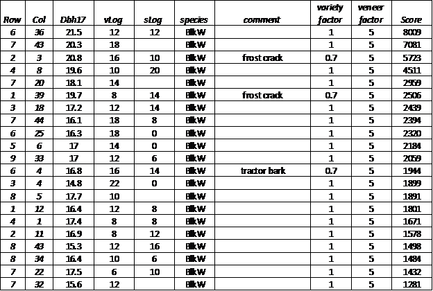
List of Trees Sorted by Descending Value Score
Chapter 7. Required Header Information and Save .csv File rev 01 2017 Jun 27
Four required items of header information are entered as item 1 of the top 4 records of the spreadsheet. The Thinning Simulator program looks for “Plot =” and expects to find the plot name after the “=”. The entire entry goes in column (item) 1. The plot name is passed through the program and will appear at the top of any report the program produces. The “Row Spacing =” and Column Spacing =” inputs should be obvious. The values need to be in feet. The “Hand =” controls how the plot is shown on the screen. The smallest numbered row always goes across the top of the screen. If the hand is “Right”, the column numbers are shown increasing to the right. If the display looks wrong, try “Left”. The “Acres =” entry allows the user to lock up the acreage of a plot and disable the automatic acreage calculation in the program. Over many thinnings, if edge trees are removed, the program computes a smaller acreage, and as edge tree grow and reach out further, the program computes more acreage. These acreage changes should be small effects on a large plot, but might be annoying on a small plot. If the program finds a numeric value after the “Acres =”, the value is used and the auto acreage calculation is ignored.
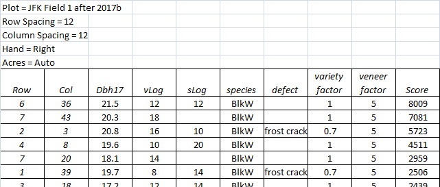
Header Items Added and Saved in .csv format
After the above required spreadsheet header records, there can be a record reserved for the spreadsheet column labels. The Thinning Simulator program looks for a record starting with the word “Row” (case insensitive) All other non-numeric records are ignored
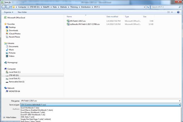
We like to create a separate file folder for each plantation plot. Now that you have the required header information and sorted tree data, save the spreadsheet twice. First save the file as a normal .xls spreadsheet. Second save the spreadsheet as a .csv file. The .csv file is a comma delimited text file that is readable by the Thinning Simulator program. To save the .csv file, go to the “File” tab and select “Save As”. A save window pops up. Go to the “Save as Type” pull-down pick list and select “CSV (comma delimited) (*.csv)”. Enter a file name you like and click the “Save” button.
![]()
Header
Items Added and Saved in .csv format
Chapter 8. Using the Thinning Simulator Software rev 01 2017 Jun 27
Startup the Thinning Simulator program and click the button labeled “Load Tree Data” at the upper left.

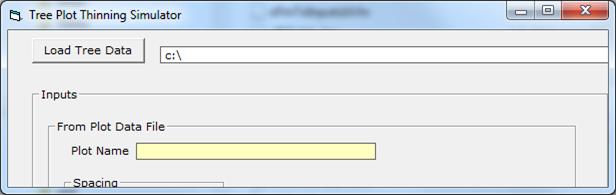
A file finder dialog form will popup to allow you to select the disk drive, directory (use double clicks), and input .csv file. It might be helpful to start out by selecting a sample .csv file included with the Thinning Simulator package. Click “OK” on the popup and the Simulator screen will be populated with input data from the highlighted .csv file.

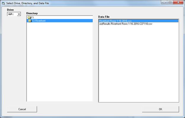
Yellow items are read or computer from the input .csv file data. Blue items are default values which are user adjustable. The tree data is displayed in the “Raw Data” window.
The “Plot Area” is either entered from the .csv file or computed from the spacings and the extents of the plot rows and columns in the input data. In the “Thinning” frame the current “Crown Competition Factor” (CFF) is computed. The CCF is a measure of tree crowding, and CCF values over 100% generally mean overcrowding and suppressed tree growth rate. “Basal Area” is another common measure of tree density, which is shown for reference. The “Growth Rate” is computed from the field observation that Black Walnut begins to be suppressed at 80% CCF and growth is slowed by 4% for every 10% increase in CCF.
The only other user adjustable item is the “Min Salable DBH”, which is defaulted to 14.5 inches. Trees to be removed larger than this number are marked “sell” rather than “cull”

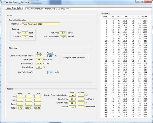
Click the “Compute Tree Selection” button to run a thinning case.
A full screen display of the plantation plot will appear the circle (tree) diameter is proportional to the tree DBH. Green trees are to be saved, blue trees are to be sold, and yellow trees are to be culled. The display flickers as the program makes multiple run until it gets the CCF of the “saved” trees about equal the CCF target.
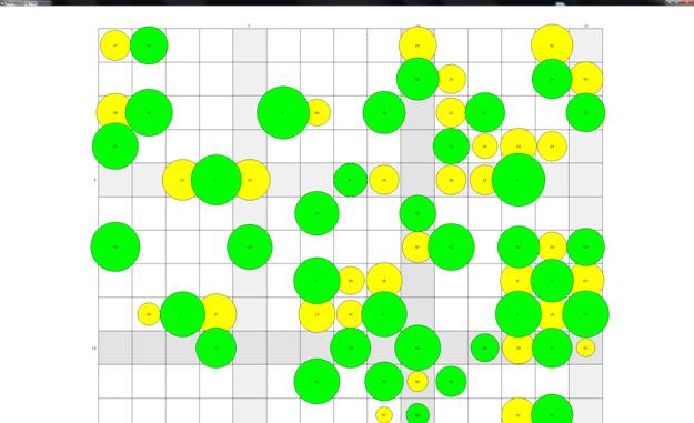
It is suggested that you try several “Target CFF” values to see the affect of different thinning intensities. It takes trees a few years to take advantage of new canopy openings. Also multiple light thinnings may allow some trees to reach the usable diameter before being removed.
After determining the desired Target CFF, click the “Save Report to File” button at the bottom to create a report .csv file. The Simulator program automatically puts the results program in the same folder with the input file. A file name is created starting with “zzzResults”, then the input file name, then “CCF”, then the numeric value of the CCF target, and finally “.csv”. If the file already exists, it is overwritten. The report .csv file can be opened as text and printed or opened as a spreadsheet.
Chapter 9. Marking and Removing Cull Trees.
With the Thinning Simulator printout report in hand, head out for your overcrowded plot. Take along some means of clearly marking the cull trees, preferably bright plastic ribbon. We prefer the ribbons. Whilst placing the ribbons, is a good time for a “sanity” check, in case an error has snuck in at some point along the process. Look at the adjacent trees and spot the better tree that eliminated the one you are marking. If you are marking the best tree around, there must be a mistake. Before you move a ribbon check your original data collection and be sure to look up in the canopy. Sometimes the crowns tell a different story than the stems. Our “sanity rule states “We can move a ribbon to an uglier unmarked adjacent tree, but we can not just pocket the ribbon. Somebody has to go.
After the cull ribbons are all in place, it is time for the actual thinning. The actual work can’t be put off much longer. We much prefer killing culls trees in-place to cutting them down. Felling heavy live trees often causes damage to the to the crop trees that are being saved. Standing killed trees gradually lose their limbs and much of their water and weight. When they are finally cut or just fall, they weigh much less, and the surrounding crop trees have become stronger.
There are several methods and a lot of information available on how to kill standing trees. Many Timber Stand Improvement (TSI) operators use frilling and herbicide as described on the “Pathway” label. In our plantation setting, we use a slightly modified approach. We girdle the cull trees. In a year or two the original tree dies and in the process produces a lot of sprouts. When the tree has dried out, (but before it rots), we cut it down for firewood. When these dry trees hit the ground most of the limbs go flying. We cut off the stump and sprouts too just above ground level. In mid-summer we brush hog and carefully go over the stumps. In a few years the stumps rot and the sprouts give up.
Chapter 10. When to Thin Again ______________________________
Now, having gone through the entire thinning process, you should be more interested in the growing value of your tree plot and the general outcome of the thinning. Only slight improvements should be expected in the vertical direction of the remaining trees. Boles will straighten slightly and defects become buried by new annual layers. The measurable response to thinning should be in the annual diametrical growth. Hopefully the growth rate before the thinning hadn’t been slowed too much and good growth can continue without suppression. If tree growth had been suppressed then the growth rate should rebound as the tree crowns expand into the opened canopy areas. A closing canopy is an easy sign that it is time for another thinning.
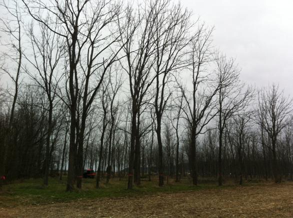
A Recommended Thinning for CC Schoolyard
As trees get bigger they want more room and become more crowded. Without intervention, the crowding and CCF number naturally and continuously increases. The long term goal should be to achieve and maintain a CCF of between 80% and 100%, which allows an unsuppressed growth rate. For severely overcrowded plots, it would be better to get to the optimum density in multiple thinning steps so as not to make such large canopy openings. The graph above shows the CC-Schoolyard overcrowded plot currently at 327 trees per acre and a CCF around 200%. Each tree is getting around half of the annual volume growth allowance it could handle. The recommended thinning removes about 1/3 of the trees and takes the tree density to 189 trees per acre and a CCF of around 150%. The thinning line ends up about an inch larger, because smaller trees tend to be removed thus increasing the average DBH for the plot. The canopy openings created should nearly close in a few years and a second thinning should have a target CCF of 80%.
Appendix A - - - Crown Competition Factor (CCF) Explained rev 01 2018 Jan 10
The Crown Competition Factor (CCF) is a measure of tree crowding widely used by foresters. The CCF is based on the following premise: A tree growing out in the open is free to grab all the sunlight it can manage. Open grown tree's growth-rate is limited by water, nutrition, genetics, whatever, but not competition for sunlight. So a forest tree given the same crown area should also grow at a rate unrestricted for want of sunlight. So 1000s and 1000s of open growth trees had their trunk diameters (DBH) and crowns areas measured, and all that data was fitted by a formula and published as a usable table of Maximum Crown Areas (MCA) numbers by the US Forest Service. The units of measure for the MCA numbers are cleaver, but a little strange. The MCA numbers are in percent of an acre, so a tree whose diameter indicates that should have 435.6 square feet (1% of an acre) of crown space, has a table MCA value of 1.0%. If you had exactly 100 such trees on an acre, the CCF for that acre would be a perfect 100% If you had 110 such trees on an acre, the CCF would be 110%, that is, 10% overcrowded.
The US Forest Service table is based on the approximation that a Maximum Crown’s Diameter (not area) is MCD (feet) = 5 + 2 x DBH (inches). The area of such a circle is about MCA = .007 x DBH^2 + .04 x DBH
A Missouri plantation owner, Michael Williams, has noticed that the above formulas are quite a ways off for very large trees – like the state champions. He suggest: MCA (1% acre) = 0.052978 X DBH ^ 1.3506, which gives the same result at 12 inch DBH and is a better data fit for very large trees. The Thinning Simulator program needs to work for any size of trees, so the Williams formula is used for trees over 12 inches DBH.
Appendix B - - - Tips on Making a Permanent Coordinate System rev 01 2017 Jun 18
Making a permanent coordinate system is one of those things that sounds easy. From experience we have found that it is a good idea to mark out the system temporarily before making the markers permanent. If you value a friendship or spouse, you might want to do this alone.
1. Get a few rolls of bright plastic ribbon all the same color, felt tip markers, some tall stakes and a hammer.
2. Mark a tree with a ribbon on every 10th row in every 10th column.
3. Write the row and column numbers on the ribbon with a felt tip pen.
4. If there is no tree at the 10th, 10th intersection, drive a tall stake and mark it similarly.
5. When the entire plot has been laid out, double check that things sort-of line up in both directions.
After you have moved the tapes to the correct trees and are satisfied with the temporary layout, you can make the permanent markers. You can paint a ring up high around each 10th, 10th tree and paint the tree coordinate below. Marking paint fades in a few years and will need to be repainted. The ribbon and paint color used to layout the coordinate system should be reserved. Use a different color to mark trees for other reasons, such as culls.
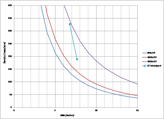
We painted numbers on pre-painted aluminum flashing with implement paint and used aluminum nails to fasten the signs to locust stakes. These signs are still in good shape after 20 years, but our stakes were either too short, or our weeds are too tall. We wanted the numbers as big as possible, so we left off the zeros. In the photo, “14” means row 140.
John Deere Yellow after 15 years
The Case of Un-Equal In-Row Spacing
We have encountered some cases where trees were planted in nice rows, but were not equally spaced within the rows. The problem was assigning a column numbers to the trees. Tree crowns in the canopy are never perfect circles, so a few feet confusion in the stem location is not serious. We suggest the following method:
Start in a corner if possible. Layout a base column line that crosses all the rows at close to 90 degrees. The base line might be a fence or a field edge. For a large plot layout more base lines at 500 foot intervals and parallel to the first base line. This will complete the layout thanks to the future use of a land measuring wheel.
To collect data, zero the wheel at the base line and proceed along a row. Stop at each tree and use the wheel footage reading as the tree column coordinate. When reaching the 500 foot line the wheel should read within a few feet of 500. Always record the wheel reading at the 500 foot line in case coordinates need to be pro-rated. Errors larger than 6 feet should probably be corrected later. To go further along the row, re-zero the wheel at the 500 foot line, adding 500 to each reading thereafter.
After data entry, analysis, and report generation, you will return to the field with ribbon to mark trees to be removed. Again zero the wheel at the base line and proceed as during data collection. It is easy to flag two rows at once. If the cull list says to remove the tree at row 2, column 127, watch the wheel counter and stop at 127. There should be an ugly tree there in row 2.
Appendix C- - - Tips on Collecting Field Data rev 01 2017 Jun 23
Our early attempts at field data collection used the data form designed by Dr. Walter Beineke. Dr. Beineke’s form consisted of one page per tree and was designed to identify the very best Black Walnut trees in North America. It took us 2 hours to do one row and we had 200 rows. Not exactly what was needed here. We eliminated everything we could and reduced the form to the example shown at the beginning of Chapter 2, which is designed for doing two rows together.
The measurement campaign should be conducted while the leaves are off the trees. In the preceding fall, brush-hog the plot in both directions so, that during next winter’s survey, you can focus on trees and not have to wade through weeds and briars. The measurement process can still be more than a little cumbersome for one person. It takes two hands to use a pi tape and two hands to write on a clipboard, plus we had a height stick. We finally developed a method that moves right along:
Next winter find two helpers. Liz Jackson has made the splendid suggestion to involve your grandkids. You are going to need them anyway to do the spreadsheet. One person measures the DBH with a pi tape. One person estimates the potential veneer and saw log lengths (No height stick. Always use the same person for length estimates. This is a tree against tree contest, not a tally). The third person is the clipboard holder and data recorder. Everybody should agree on each tree’s coordinates. Getting a coordinate wrong can cause a lot of trouble, like sawing down the wrong tree. Everybody also helps the length estimator spot major cat-faces and other serious defects. After a few measurements, the team will settle in to which person best fits each role.
There is some art to estimating the length of potential veneer and saw logs. Visualize a veneer log starting about a foot above the ground or just above a frost crack. Continue up the tree bole until a showstopper is encountered. A showstopper might be a limb, stub, or catface greater than 2 inched in diameter. Other stoppers might be a crotch, a crook, or a mass of bird pecks. The veneer potential segment must be at least 6 feet long. For veneer quality, the bark needs to look nice. Luckily the demand for Black Walnut veneer is always high, so the quality requirements continually slacken. Saw logs need to be straight segments at least 6 feet long for Black Walnut (8 feet for other species) continuing up to a really major defect, like a crotch. Log estimations are tough and have an important impact. I have found, working by myself that it is better to go fast and do the whole length campaign in one quick session. To make it go fast, I measure all the DBHs first, then go back and do all the lengths. I don't want my standards to change midstream. If my standards are consistent, good trees will still beat out lesser trees, even if I'm off by 50%.
After you circle a few trees looking up, you will be lucky to be on the same rows, so park your Kubota RTV 1100 at the end of the two rows being measured as an expensive temporary landmark.
![]()
Here are a few words on how to deal with some special cases:
F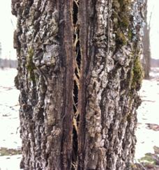 ROST CRACKS usually start at ground level and
proceed up 4 to 10 feet. They favor the south side of the tree, but can be in
any direction. They heal over in the summer and are torn open during the
bitter cold of winter, allowing all kinds of unwanted vermin into the tree.
Internal damage does not extend above the top of the crack, but there is
essentially no timber value below the top of the crack. For tree value,
discount the entire cracked area and only count lengths above the crack. It
would be unwise to save a cracked tree in a final thinning (past age 40), since
it will likely be a hollow tree in old age. In addition to the length
discount, such damaged trees should be treated as a low value variety. I
always give them a 0.7 variety factor
ROST CRACKS usually start at ground level and
proceed up 4 to 10 feet. They favor the south side of the tree, but can be in
any direction. They heal over in the summer and are torn open during the
bitter cold of winter, allowing all kinds of unwanted vermin into the tree.
Internal damage does not extend above the top of the crack, but there is
essentially no timber value below the top of the crack. For tree value,
discount the entire cracked area and only count lengths above the crack. It
would be unwise to save a cracked tree in a final thinning (past age 40), since
it will likely be a hollow tree in old age. In addition to the length
discount, such damaged trees should be treated as a low value variety. I
always give them a 0.7 variety factor
Frost Crack at -2 degrees F. showing all last summer's healing being ruined.
BARK DAMAGE caused by antler rub, tractor rub, or mower rub may heal over depending on the size of the damage. In any case the area should be disqualified for veneer length. If the damage is large, it should be handled like the frost crack above. If you are thinning, it is probably too late for coppicing. Trees with damage more than 3 inches wide should be treated as a low value variety.
LEAN has been a showstopper for veneer use in the past, however new methods at veneer plants accommodate the stresses associated with the off-centered-heart. In essence, a reasonable lean is no longer a defect.
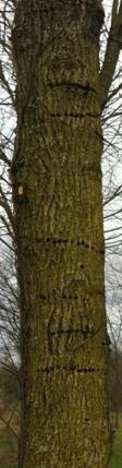 BIRD PECKS come in two flavors and veneer
buyers are uncanny at spotting them on log bark surfaces. The sap sucker pecks
are in a horizontal row and easy to see (left and below). The more conniving
kind is in the groves between bark ridges. They continue outward with cambium
growth and are difficult to see. It is unlikely that either of these defects
will be accepted for veneer use.
BIRD PECKS come in two flavors and veneer
buyers are uncanny at spotting them on log bark surfaces. The sap sucker pecks
are in a horizontal row and easy to see (left and below). The more conniving
kind is in the groves between bark ridges. They continue outward with cambium
growth and are difficult to see. It is unlikely that either of these defects
will be accepted for veneer use.
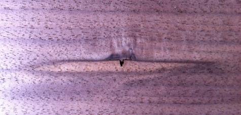 |
Bird peck in bark and veneer
CROOK can be a problem or no problem at all. No mill wants a log with a crook, so if possible loggers buck stems right through crooks to yield straight logs on each side. To count log length above or below a crook, the straight segment must be at least 6 feet long for Black Walnut and 8 feet for other species.
SWEEP in a tree stem is a long curve. Veneer is out of the question and saw mills will give huge tally deductions. To make it simple, consider the entire sweep area as valueless.
LIMB CUT / CAT-FACE / BUMP: Judging these defects is the main occupation of the quality cruiser. A healed-over and buried defect is not acceptable for veneer use if the is visible at harvest time. I am comfortably sure that a 1 inch branch removal wound on a 4 inch tree will become bark invisible in a 30 inch diameter log. I’m guessing that a catface that is hard to see at 10 inches will also disappear.
SPECIAL TREES, like heavy nut producers, nut cultivars, figured varieties, or a seedling grown from nuts collected by George Washington, can be saved and given special treatment by the Thinning Simulator program. Make a field note of any tree you want to receive such special treatment – good or bad. When computing tree value scores in the working spreadsheet, just type in some appropriate variety factor. The high score will move your pet tree to the top of the list when sorted and it will be given first choice for canopy space.
Appendix D - - - Formula for Computing Relative Tree Value rev 02 2018 Feb 17
Saw Logs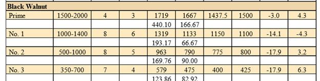
A Black Walnut plantation doesn’t make much economic sense unless it produces veneer quality timber. Foresters have claimed that 80% of a tree’s value is in the butt log. The percentage would be even higher in the case of veneer quality trees, which are our objective. The following formula is sensitive to the importance of veneer quality. At times growers have other objectives and should adapt their own relative value formula proportional to their objective.
This formula for relative tree value is only used to arbitrate arguments between adjacent trees. Multiplying all tree values by 5 or pi or dividing by 12 will not change the ranking of a tree or the outcome of an argument. The relative tree value formula has these parts.
1. Area Basal A = pi * D2 / 4, where D is the DBH.
2. Volume Cylindrical Veneer VV = A * LV, , where LV is the length of a potential veneer log
3. Volume Cylindrical Saw log VS = A * LS , where LS is the length of a potential saw log
4. Tree Volume Score S = FV * VV + VS , where FV is a veneer factor, typically about 5
Veneer logs are worth about 5 times more than saw logs. All simple so far. I know logs are not true cylinders, but changing the formula to cones or Doyle scale wooden affect the rankings.
If a beautiful small diameter tall tree had the exact same volume as a short fat tree, some people might like to favor the skinny tall tree, because it has more potential. To accommodate favoring small diameters there is an ugly adjustable multiplier.
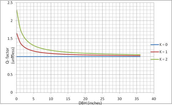
5. Small Diameter Kindness Q = K * (exp(1/(2+D)) - 1) + 1 , where K is the adjustment Knob.
Setting K = 0 gives Q = 1 for any diameter. I personally like K = 1, and Q always approaches 1 for big diameters.
6. The Final Relative Tree Value is R = S * Q * FS, where FS is a variety or defect or species factor.
To arrive at your personal value for K, try K = 1 and sort the trees in descending R score. Look down the sorted list of DBHs and Lengths. If you agree with the sorted order, cool. If you think it is favoring small tall trees too much reduce or zero K, and re-sort.
Appendix E - - - Simulating Average Tree Growth rev 01 2017 Jun 23
Our early attempts at field data collection used the data form designed by Dr. Walter Beineke. Dr. Beineke’s form consisted of one page per tree and was designed to identify the very best Black Walnut trees in North America. It took us 2 hours to do one row and we had 200 rows. Not exactly what was needed here. We eliminated
Appendix Y Possible Uses for Undersized Logs and Waste Material.
Firewood
Salt and Pepper Items
Premium Black Walnut Biochar
Appendix Z The Thinning Simulator Algorithms and Mathematics